Earlier this year, I got a puppy and always wondered how large she would grow to be. From the moment she came home, I have been weighing her consistently to get a feel for how fast she was growing and guess her weight at maturity. Based on her type, I thought she might grow to 45 lbs, but it was hard to tell where she might stop during the rapid growth phase of puppyhood. My dog’s growth has started to slow down, so I figured I might start to predict my dog’s weight at maturity. I thought it would be fun to write up that process and share it with you all! We will use both Bayesian inference with pymc and non-linear least squares and compare results.

Growth Models
I am sure there is a lot of research around dog or mammal growth curves, and which models are most appropriate. But, I wanted to compare a few models, so I selected three growth models from GraphPad’s website:
Logistic Growth: \[ f(t) = \frac{Y_M \cdot Y_0}{(Y_M-Y_0) \cdot e^{-k \cdot t} +Y_0} \]
Gompertz: \[ f(t) = Y_M \cdot \left( \frac{Y_0}{Y_M}\right)^{e^{-k \cdot t}} \]
Exponential Plateau: \[ f(t) = Y_M - (Y_M-Y_0) \cdot e^{-k \cdot t} \]
These three models have the same three parameters that are used differently in the equations:
\(t\) : independent time variable. This will be the age of the dog in weeks.
\(Y_0\) : Initial weight at \(t\) = 0 (birth). You can see that at \(t\)=0, the exponential terms are raised to zero (which is equal to 1), and the equations all collapse to \(Y_0\).
\(Y_M\) : Maximum asympototic weight. You can also see that at \(t\) = \(\infty\), the exponential terms are raised to negative infinity, which zeroes out the term, leaving \(Y_M\).
\(k\) : growth rate during exponential phase. All three equations conserve \(e^{-kt}\), but the placement of this term alters how fast the growth really is.
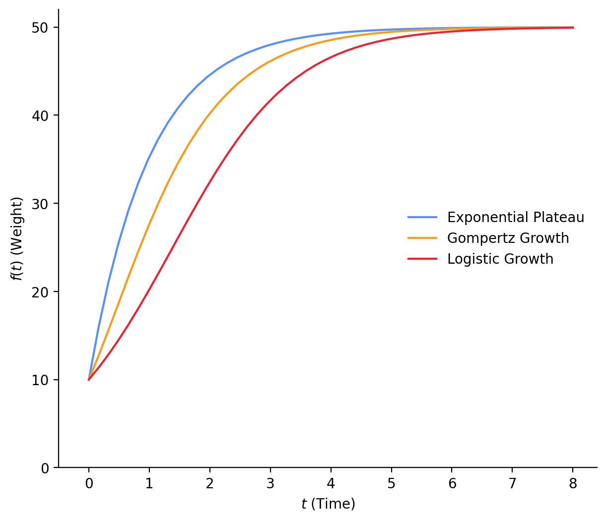
For comparison, here are all three curves with \(Y_0\) = 10, \(Y_M\) = 50, and \(k\) = 1 (Figure 1). You can see that Logistic Growth starts growing more slowly than the rest, picks up, but still grows slower than the others. Exponential Plateau starts growing much faster than the rest. I am not sure which of these models will fit our data, but let’s find out! Next, we’ll start to build our Bayesian models.
Bayesian Inference
In this section, we have the following objectives:
- Outline Bayesian model
- Select priors that we will use in our Bayesian models for the growth curves
- Check the priors can give us sensical models (without data)
- Run Bayesian inference models
- Evaluate the quality of posteriors
- Evaluate the quality of our models with some reserved recent data
- Determine when we can be more certain which model is right, and what age my dog will reach her final weight
Bayesian Model
The bulk of this post is devoted to using Bayesian methods to estimate the parameters of our growth curves and make inferences. So, we will need to start building a Bayesian model (that will be similar for the three curve models mentioned above). We’re going to assume that a weight predicted by a growth curve is an idealized weight, but our observations will be distributed around that weight. So given a particular age (\(age_i\)), there is an ideal/average weight (\(\mu_i\)), from which many individual \(weight_i\) can be sampled.
\[ \begin{aligned} weight_i \sim&\ \operatorname{Normal}(\mu_i,\,\sigma)\\ \\ \end{aligned} \]
\(\sigma\) is the standard deviation of this distribution and indicates the nature of the natural variance or error in our measurements.
We already know that \(\mu_i\) is governed by our growth curve models and input ages, but the other parameters of the growth curves are also sampled from distributions. These are our priors, which we will reason through specifying in the next section.
\[ \begin{aligned} weight_i \sim&\ \operatorname{Normal}(\mu_i,\,\sigma)\\ \\ \mu_i =&\ \operatorname{Curve\_Model}(age_i,\,Y_M,\,Y_0,\,k)\\ \\ Y_0 \sim&\ ?\\ \\ Y_M \sim&\ ?\\ \\ k \sim&\ ?\\ \\ \sigma \sim&\ \operatorname{Exponential}(\lambda =\ 1)\\ \\ \end{aligned} \]
Bayesian inference status:
- Outline Bayesian model
- Select priors that we will use in our Bayesian models for the growth curves
- Check the priors can give us sensical models (without data)
- Run Bayesian inference models
- Evaluate the quality of posteriors
- Evaluate the quality of our models with some reserved recent data
- Determine when we can be more certain which model is right, and what age my dog will reach her final weight
Priors
We will be fitting some models to arrive at our best estimates of the \(Y_0\), \(Y_M\), and \(k\) terms. I’ll use the same priors for these parameters for each of the three models. To start, let’s pick a prior for \(Y_0\).
\(Y_0\)
Again, this is the weight of the puppy at birth (Aside, I don’t really care about learning the birth weight, but it’s part of the model. I won’t be upset if our model doesn’t cover the weight at younger ages well). We know \(Y_0\) must be positive and will be relatively close to zero. From some online searches, puppies in general can be anywhere from 0.25 lbs to 2.25 lbs at birth. Given our proximity to 0, let’s use a Gamma distribution as a prior for \(Y_0\).
We can use a midpoint of this birthweight range as our mean (\(\mu\) = 1.75 lbs), and assume this range corresponds to ± 3 standard deviations (\(\sigma\) = 0.5). This will break down a bit because the Gamma distribution is not symmetric, but it’s fine for our purposes. We will use the \(\alpha\) (shape) and \(\beta\) (rate) parametrization of Gamma, and can solve for those parameters from this mean and standard deviation:
\[ \begin{aligned} \alpha &= \frac{\mu^2}{\sigma^2} = \frac{1.75^2}{0.5^2} = 12.25 \\ \\ \beta &= \frac{\mu}{\sigma^2} = \frac{1.75}{0.5^2} = 7 \end{aligned} \]
The probability density function of this prior is below with the others (Figure 2).
\(Y_M\)
For this dog type, I’m led to believe that 45 lbs is a decent guess for final weight. I could imagine this final weight ranging anywhere from 37.5 to 52.5 lbs, so let’s use that range as ± 3 standard deviations and use a Normal distribution with mean of 45 and sigma of 2.5 for our \(Y_M\). This value should also be positive, but it’s far enough away from 0 that I’m not worried about getting negative numbers from this distribution. The probability density function of this prior is below with the others (Figure 2).
\(k\)
I know much less about \(k\). My intuition is that it should be small, on the order of 1? In our case, it should also be positive, so let’s use a Gamma distribution again. We can set its mean at 1 (\(\mu\) = 1) and give it a standard deviation of 1 (\(\sigma\) = 1).
A Gamma distribution with \(\alpha\) = 1 is an Exponential distribution! The Exponential distribution is a special case of the Gamma distribution.
\[ \begin{aligned} \alpha &= \frac{\mu^2}{\sigma^2} = \frac{1^2}{1^2} = 1 \\ \\ \beta &= \frac{\mu}{\sigma^2} = \frac{1}{1^2} = 1 \end{aligned} \]
The probability density function of this prior is below with the others (Figure 2). You can see now that this really does have an Exponential distribution that is different from the typical Gamma distribution.
Visualize Priors
We can use the python package preliz (from the team behind arviz) to easily plot these priors below. You could also use this package to help pick the priors more interactively.
import arviz as az
import matplotlib.pyplot as plt
import numpy as np
import pymc as pm
from cycler import cycler
from matplotlib import rcParams

%config InlineBackend.figure_format = 'retina'
%load_ext watermark

petroff_6 = cycler(color=["#5790FC", "#F89C20", "#E42536", "#964A8B", "#9C9CA1", "#7A21DD"])

rcParams["axes.spines.top"] = False
rcParams["axes.spines.right"] = False
rcParams["axes.prop_cycle"] = petroff_6
fig, axes = plt.subplots(3, 1, figsize=(7, 4), layout="constrained")
plt.sca(axes[0])
pz.Gamma(12.25, 7).plot_pdf(pointinterval=True, legend=False)
plt.xlabel("$Y_0$")
plt.sca(axes[1])
pz.Normal(45, 2.5).plot_pdf(pointinterval=True, legend=False)
plt.xlabel("$Y_M$")
plt.sca(axes[2])
pz.Gamma(1, 1).plot_pdf(pointinterval=True, legend=False)
plt.xlabel("$k$");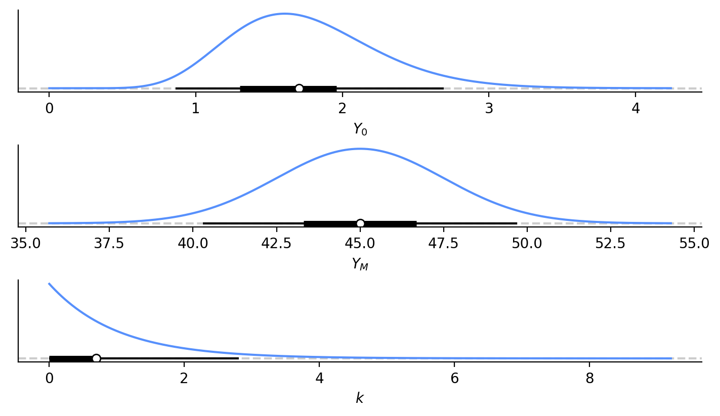
Bayesian inference status:
- Outline Bayesian model
- Select priors that we will use in our Bayesian models for the growth curves
- Check the priors can give us sensical models (without data)
- Run Bayesian inference models
- Evaluate the quality of posteriors
- Evaluate the quality of our models with some reserved recent data
- Determine when we can be more certain which model is right, and what age my dog will reach her final weight
Prior Predictive Check
With these priors in hand, for all three models, let’s perform a prior predictive check to see if we would get reasonable parameter estimations without seeing any data. Since we are choosing to use the same priors for all three models, we can share the same prior predictive sampling for all three models. We’ll generate 50 samples, build growth curves using the \(Y_0\), \(Y_M\), and \(k\) from each of the 50 samples and see if our growth curves look reasonable and valid. (Figure 3)
RANDOM_SEED = 14
rng = np.random.default_rng(RANDOM_SEED)

with pm.Model() as model_priors:
    ym = pm.Normal("ym", 45, 2.5)
    y0 = pm.Gamma("y0", 12.25, 7)
    k = pm.Gamma("k", 1, 1)

    idata_priors = pm.sample_prior_predictive(samples=50, random_seed=rng)
# Convert growth curves into python functions
def logistic_growth(x, ym, y0, k):
# https://www.graphpad.com/guides/prism/latest/curve-fitting/reg_logistic-growth.htm
return ym * y0 / ((ym - y0) * np.exp(-k * x) + y0)
def gompertz(x, ym, y0, k):
# https://www.graphpad.com/guides/prism/latest/curve-fitting/reg_gompertz-growth.htm
return ym * (y0 / ym) ** (np.exp(-k * x))
def exp_plat(x, ym, y0, k):
# https://www.graphpad.com/guides/prism/latest/curve-fitting/reg_exponential-plateau.htm
return ym - (ym - y0) * np.exp(-k * x)__, axes = plt.subplots(3, 1, figsize=(7, 8), sharex=True, sharey=True)
weeks_range = np.arange(0, 81, 1)
x = xr.DataArray(weeks_range, dims=["plot_dim"])
prior = idata_priors.prior
y = logistic_growth(x, prior["ym"], prior["y0"], prior["k"])
axes[0].plot(x, y.stack(sample=("chain", "draw")), c="k", alpha=0.4)
axes[0].set_title("Logistic Growth")
axes[0].set_ylabel("Weight (lbs)")
prior = idata_priors.prior
y = gompertz(x, prior["ym"], prior["y0"], prior["k"])
axes[1].plot(x, y.stack(sample=("chain", "draw")), c="k", alpha=0.4)
axes[1].set_title("Gompertz Growth")
axes[1].set_ylabel("Weight (lbs)")
prior = idata_priors.prior
y = exp_plat(x, prior["ym"], prior["y0"], prior["k"])
axes[2].plot(x, y.stack(sample=("chain", "draw")), c="k", alpha=0.4)
axes[2].set_title("Exponential Plateau")
axes[2].set_xlabel("Age (weeks)")
axes[2].set_ylabel("Weight (lbs)")
plt.tight_layout()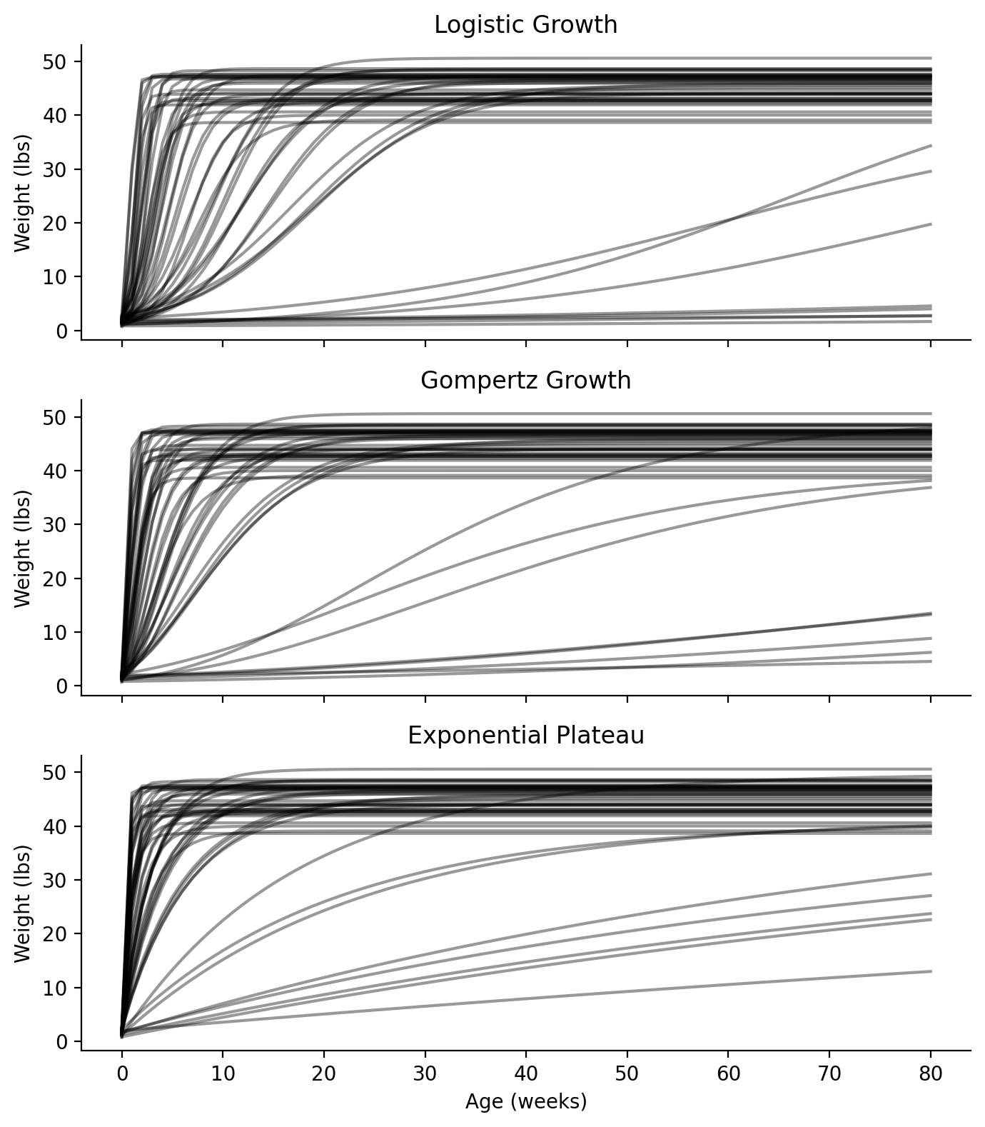
Looking at the prior predictive checks for all three models, we can see that they mostly seem to plateau around 40 - 50 lbs (we already knew that from Figure 2). But we can also see the range of different growth rates. We did give a wide prior, so our data will be helpful here to help identify the most probable rates. Some of these curves seem to plateau within 10-20 weeks (2.5-5 months), which seems unlikely. I’m guessing \(k\) will end up on the lower end of our prior.
Bayesian inference status:
- Outline Bayesian model
- Select priors that we will use in our Bayesian models for the growth curves
- Check the priors can give us sensical models (without data)
- Run Bayesian inference models
- Evaluate the quality of posteriors
- Evaluate the quality of our models with some reserved recent data
- Determine when we can be more certain which model is right, and what age my dog will reach her final weight
Final Bayesian Model
We now have a final Bayesian model we can use for each curve model. We can now load our data and start building our Bayesian models in pymc.
\[ \begin{aligned} weight_i \sim&\ \operatorname{Normal}(\mu_i,\,\sigma)\\ \\ \mu_i =&\ \operatorname{Curve\_Model}(age_i,\,Y_M,\,Y_0,\,k)\\ \\ Y_0 \sim&\ \operatorname{Gamma}(\alpha_{Y_0} =\ 12.25,\,\beta_{Y_0} =\ 7) \\ \\ Y_M \sim&\ \operatorname{Normal}(\mu_{Y_M} =\ 45,\,\sigma_{Y_M} =\ 2.5)\\ \\ k \sim&\ \operatorname{Gamma}(\alpha_{k} =\ 1,\,\beta_{k} =\ 1) \\ \\ \sigma \sim&\ \operatorname{Exponential}(\lambda =\ 1)\\ \\ \end{aligned} \]
Data Inspection
So far, we haven’t touched the data at all. We have collected some different growth models and created some priors for the growth model parameters from our pre-existing knowledge or best guesses. Now, we can load the data and finish building our Bayesian models in pymc.
from pathlib import Path

import pandas as pd

DATA_DIR = Path.cwd() / "data"

df = pd.read_csv(DATA_DIR / "dog-weight.csv")
df["Age (weeks)"] = df["Age (days)"] / 7
df = df[["Age (days)", "Age (weeks)", "Weight (lbs)"]]
I collected this data since my dog was 9.5 weeks old, and I measured her weight roughly two times a week. The data shown in this post includes up to 38.5 weeks old; hopefully in a few months we’ll be able to use the subsequent data to see which model was truly the best. The weight was measured after a morning walk, but before breakfast, with the same scale, so hopefully the data is as consistent as reasonably possible.
Our goal is to pick a model that fits our current data as well as future months’ weight data. I will reserve the last 4 weeks of this data to validate these models. Hopefully the remaining data captures enough of the slowdown in growth to give an idea of the final weight and ideal model.
pd.concat((df.head(), df.tail()))| Age (days) | Age (weeks) | Weight (lbs) | |
|---|---|---|---|
| 0 | 67 | 9.571429 | 13.1 |
| 1 | 71 | 10.142857 | 13.2 |
| 2 | 74 | 10.571429 | 13.6 |
| 3 | 77 | 11.000000 | 14.2 |
| 4 | 81 | 11.571429 | 15.2 |
| 48 | 256 | 36.571429 | 39.6 |
| 49 | 259 | 37.000000 | 39.2 |
| 50 | 263 | 37.571429 | 39.0 |
| 51 | 266 | 38.000000 | 39.6 |
| 52 | 270 | 38.571429 | 40.2 |
# Label data within the final four weeks as Test set, rest is Train
df["Set"] = ""
max_age = df["Age (weeks)"].max()
df.loc[df["Age (weeks)"] >= (max_age - 4), "Set"] = "Test"
df.loc[df["Age (weeks)"] < (max_age - 4), "Set"] = "Train"
df_train = df.loc[df["Set"] == "Train"]
df_test = df.loc[df["Set"] == "Test"]
print(
f"Train Set Size: {df_train.shape[0]}, "
+ f"Train Set Percentage: {df_train.shape[0]/df.shape[0]:.1%}"
)
print(
f"Test Set Size: {df_test.shape[0]}, "
+ f"Test Set Percentage: {df_test.shape[0]/df.shape[0]:.1%}"
)Train Set Size: 44, Train Set Percentage: 83.0%
Test Set Size: 9, Test Set Percentage: 17.0%__, ax = plt.subplots(figsize=(7, 5))
sns.scatterplot(x="Age (weeks)", y="Weight (lbs)", hue="Set", data=df, ax=ax)
ax.set_xlim(left=0)
ax.set_ylim(bottom=0);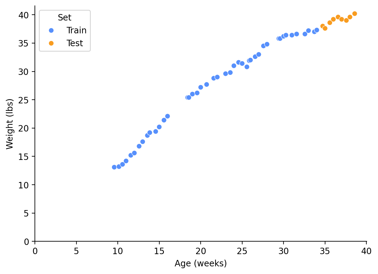
Build the Bayesian Models in pymc
We’ll now build the Bayesian models we outlined in Final Bayesian Model section using pymc. Every line in our model has been translated to a line of code.
Instead of using the raw training input directly (df_train[“Age (weeks)”]), we are plugging it into pm.MutableData(). This has the benefit of allowing us to run our model once, make update the mutable input data, and run the model for a new purpose (like making predictions). This will save us a lot of effort.
Finally, pm.sample() runs our model with a specified number of tuning steps, samples to collect, and parallel chains.
with pm.Model() as model_gompertz:
    ym = pm.Normal("ym", 45, 2.5)
    y0 = pm.Gamma("y0", 12.25, 7)
    k = pm.Gamma("k", 1, 1)
    weeks = pm.MutableData("weeks", df_train["Age (weeks)"], dims="obs_id")
    weight = df_train["Weight (lbs)"]
    mu = gompertz(weeks, ym, y0, k)

    sigma = pm.Exponential("sigma", 1.0)
    obs = pm.Normal("obs", mu=mu, sigma=sigma, observed=weight, dims="obs_id")

    idata_gompertz = pm.sample(tune=2000, draws=1000, chains=4, random_seed=rng)

with pm.Model() as model_log:
    ym = pm.Normal("ym", 45, 2.5)
    y0 = pm.Gamma("y0", 12.25, 7)
    k = pm.Gamma("k", 1, 1)
    weeks = pm.MutableData("weeks", df_train["Age (weeks)"], dims="obs_id")
    weight = df_train["Weight (lbs)"]
    mu = logistic_growth(weeks, ym, y0, k)

    sigma = pm.Exponential("sigma", 1.0)
    obs = pm.Normal("obs", mu=mu, sigma=sigma, observed=weight, dims="obs_id")

    idata_log = pm.sample(tune=2000, draws=1000, chains=4, random_seed=rng)

with pm.Model() as model_exp:
    ym = pm.Normal("ym", 45, 2.5)
    y0 = pm.Gamma("y0", 12.25, 7)
    k = pm.Gamma("k", 1, 1)
    weeks = pm.MutableData("weeks", df_train["Age (weeks)"], dims="obs_id")
    weight = df_train["Weight (lbs)"]
    mu = exp_plat(weeks, ym, y0, k)

    sigma = pm.Exponential("sigma", 1.0)
    obs = pm.Normal("obs", mu=mu, sigma=sigma, observed=weight, dims="obs_id")

    idata_exp = pm.sample(tune=2000, draws=1000, chains=4, random_seed=rng)
Let’s start to compare the model fits by looking at the summary of the parameter posterior distributions. For one of our models, we can generate a summary with az.summary():
az.summary(idata_log, kind="stats")| mean | sd | hdi_3% | hdi_97% | |
|---|---|---|---|---|
| ym | 39.921 | 0.475 | 39.027 | 40.799 |
| y0 | 4.460 | 0.230 | 4.033 | 4.886 |
| k | 0.139 | 0.004 | 0.131 | 0.147 |
| sigma | 0.569 | 0.065 | 0.449 | 0.689 |
For all our parameters (remember sigma is a feature of our regression, but not the growth models themselves) we have means, standard deviations (sd) and 94% highest density interval (HDI) (hdi_3% -> hdi_97%). We will use the 94% HDI as our Bayesian credible interval. Given our model and data, we are 94% certain that the true value of our parameters lies within the 94% HDI.
From this summary of the Logistic Growth model, we can see that the most likely value for \(Y_M\) is 39.9 lbs but may range between 39.0 and 40.8 lbs. We ultimately care about the comparison of the whole models, but we can aggregate these summaries for the different models and get some insight into differences between the fits.
summary_all = pd.concat(
    (
        az.summary(idata_exp, kind="stats").assign(model="Exponential Plateau"),
        az.summary(idata_gompertz, kind="stats").assign(model="Gompertz Growth"),
        az.summary(idata_log, kind="stats").assign(model="Logistic Growth"),
    )
).reset_index(names="param")
summary_all| param | mean | sd | hdi_3% | hdi_97% | model | |
|---|---|---|---|---|---|---|
| 0 | ym | 54.077 | 2.126 | 50.155 | 58.095 | Exponential Plateau |
| 1 | y0 | 1.025 | 0.298 | 0.464 | 1.573 | Exponential Plateau |
| 2 | k | 0.033 | 0.002 | 0.030 | 0.037 | Exponential Plateau |
| 3 | sigma | 1.524 | 0.203 | 1.143 | 1.888 | Exponential Plateau |
| 4 | ym | 42.725 | 0.602 | 41.586 | 43.872 | Gompertz Growth |
| 5 | y0 | 2.170 | 0.217 | 1.772 | 2.580 | Gompertz Growth |
| 6 | k | 0.093 | 0.003 | 0.087 | 0.099 | Gompertz Growth |
| 7 | sigma | 0.508 | 0.057 | 0.407 | 0.619 | Gompertz Growth |
| 8 | ym | 39.921 | 0.475 | 39.027 | 40.799 | Logistic Growth |
| 9 | y0 | 4.460 | 0.230 | 4.033 | 4.886 | Logistic Growth |
| 10 | k | 0.139 | 0.004 | 0.131 | 0.147 | Logistic Growth |
| 11 | sigma | 0.569 | 0.065 | 0.449 | 0.689 | Logistic Growth |
Let’s take this dataframe and make some simple forest plots of the means and HDI of each parameter (Figure 5). From the table above and the graphs below, we can see that for \(Y_M\), Logistic Growth and Gompertz Growth estimate similar values of 39.9 lbs and 42.7 lbs, respectively. The 94% HDI of these two estimates are close, but don’t overlap. \(Y_M\) from the Exponential Plateau model, on the other hand, is estimated to be 54.1 lbs, with an 94% HDI that spans 8 lbs.
I didn’t really care about \(Y_0\) because my purpose is to predict future weights, but there is also quite a range of dog birthweights predicted by the different models. The estimates for Gompertz Growth and Exponential Plateau are reasonable, but the Logistic Growth model estimates a birthweight of 4.5 lbs, which is extremely high!
I originally guessed that the \(k\) parameters for the model would be somewhere about 1 (for no reason), but it looks like I was off by an order of magnitude or two. Finally, sigma is indicative of the distribution of error of our observed data with respect to the fit model. sigma for the Exponential Plateau is extremely high! This is a good early warning sign that we may have a poor fit with that model.
Code
fig, axes = plt.subplots(4, 1, figsize=(7, 7))
for i, param in enumerate(["ym", "y0", "k", "sigma"]):
    plt.sca(axes[i])
    axes[i].hlines(
        y="model",
        xmin="hdi_3%",
        xmax="hdi_97%",
        data=summary_all.loc[summary_all["param"] == param],
    )
    axes[i].scatter(
        x="mean",
        y="model",
        data=summary_all.loc[summary_all["param"] == param],
        s=20,
    )
    axes[i].set_xlabel(param)
    axes[i].set_title(f"Param: {param}")
    axes[i].set_ylim(-0.2, 2.2)
plt.subplots_adjust(hspace=1)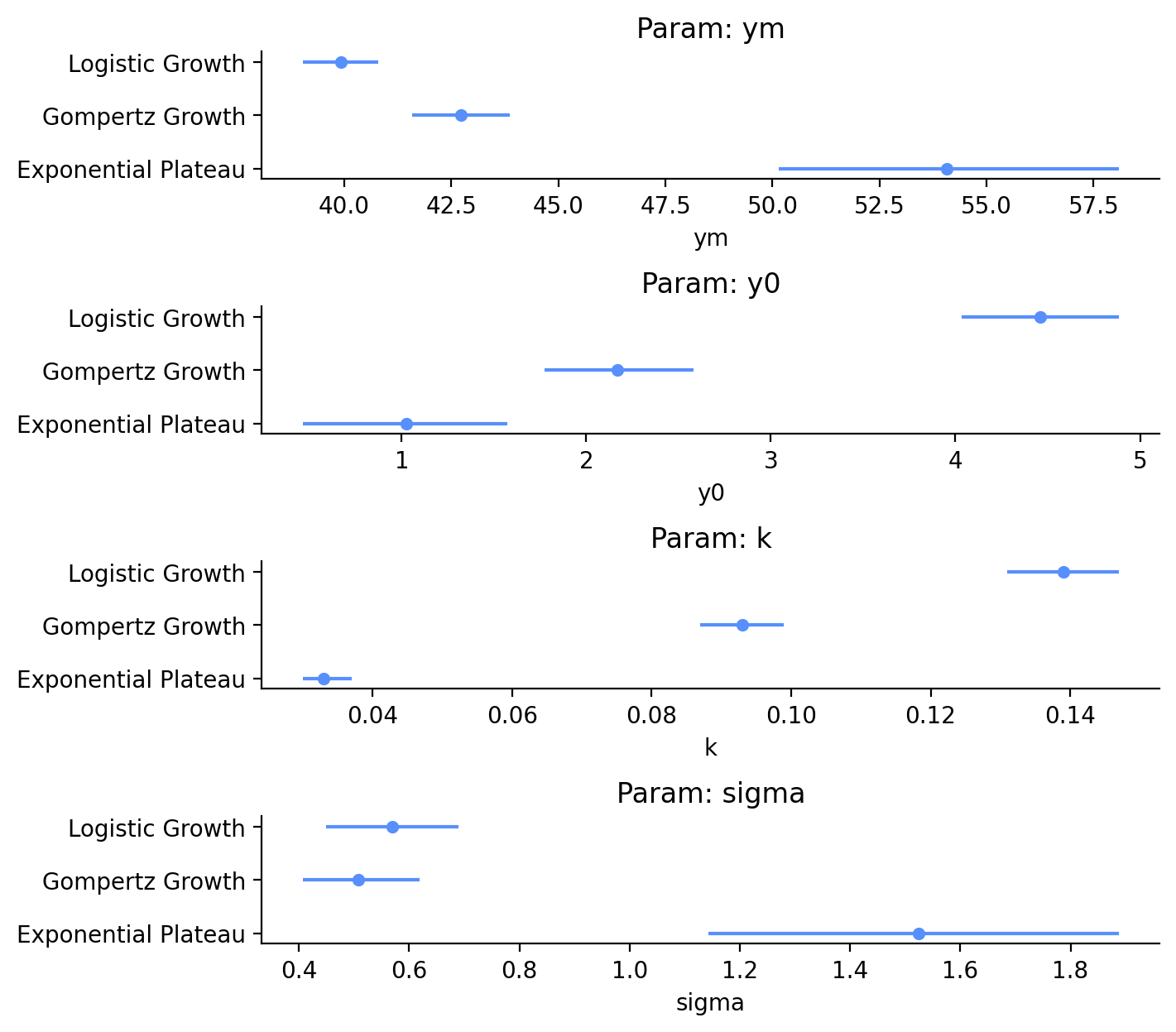
Bayesian inference status:
- Outline Bayesian model
- Select priors that we will use in our Bayesian models for the growth curves
- Check the priors can give us sensical models (without data)
- Run Bayesian inference models
- Evaluate the quality of posteriors
- Evaluate the quality of our models with some reserved recent data
- Determine when we can be more certain which model is right, and what age my dog will reach her final weight
Compare Growth Curve Posteriors
Let’s finally look at the estimates of these models, putting together the estimates of the individual parameters. We can generate posterior predictive samples using our existing models, which are built off our training data.
with model_gompertz:
    posterior_predictive_gompertz_train = pm.sample_posterior_predictive(
        trace=idata_gompertz, random_seed=rng
    )


with model_log:
    posterior_predictive_log_train = pm.sample_posterior_predictive(
        trace=idata_log, random_seed=rng
    )

with model_exp:
    posterior_predictive_exp_train = pm.sample_posterior_predictive(
        trace=idata_exp, random_seed=rng
    )
Following our Bayesian principles, instead of taking the mean values of our fit parameters, we will plot the curves using 94% HDI bands (Figure 6). Using our training data, and only looking at the range of ages covered by our training data, we can see that the Logistic Growth and Gompertz Growth models are nearly identical and seem to be a good approximation of the underlying function. The Exponential Plateau model, on the other hand, doesn’t match the underlying function. It overestimates the weight at low ages and underestimates it at higher ages. This is why sigma and the current HDI are so large.
fig, ax = plt.subplots(figsize=(7, 5), layout="constrained")
az.plot_hdi(
    x=df_train["Age (weeks)"],
    y=posterior_predictive_exp_train.posterior_predictive["obs"],
    hdi_prob=0.94,
    color="C0",
    fill_kwargs={"alpha": 0.3, "label": "94% HDI (Exponential Plateau)"},
    smooth=False,
    ax=ax,
)
az.plot_hdi(
    x=df_train["Age (weeks)"],
    y=posterior_predictive_log_train.posterior_predictive["obs"],
    hdi_prob=0.94,
    color="C1",
    fill_kwargs={"alpha": 0.3, "label": "94% HDI (Logistic Growth)"},
    smooth=False,
    ax=ax,
)
az.plot_hdi(
    x=df_train["Age (weeks)"],
    y=posterior_predictive_gompertz_train.posterior_predictive["obs"],
    hdi_prob=0.94,
    color="C2",
    fill_kwargs={"alpha": 0.3, "label": "94% HDI (Gompertz Growth)"},
    smooth=False,
    ax=ax,
)

ax.scatter(
    df_train["Age (weeks)"],
    df_train["Weight (lbs)"],
    label="Observed (training)",
    color="0.4",
)

plt.legend(frameon=False)
ax.set_xlabel("Age (weeks)")
ax.set_ylabel("Weight (lbs)")
ax.set_xlim(left=0)
ax.set_ylim(bottom=0);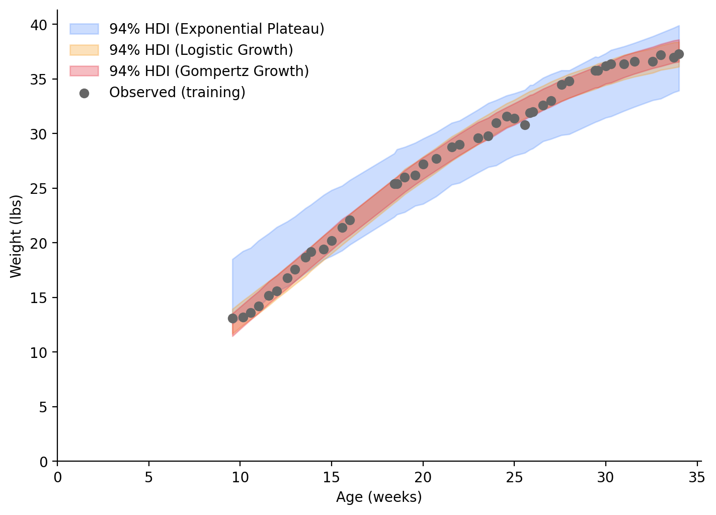
Bayesian inference status:
- Outline Bayesian model
- Select priors that we will use in our Bayesian models for the growth curves
- Check the priors can give us sensical models (without data)
- Run Bayesian inference models
- Evaluate the quality of posteriors
- Evaluate the quality of our models with some reserved recent data
- Determine when we can be more certain which model is right, and what age my dog will reach her final weight
Predict Future Dog Weights
Now, let’s see how well our models perform on the 4 weeks of recent data that we withheld from the training. We will generate samples from the posterior predictive, again. We want to get these samples based off our actual testing dataset, as well as a range of ages that will show us predicted weights in the future. This is why we used pm.MutableData() for our input age data when building the models. For each model, we can update the input data, and run pm.sample_posterior_predictive(). Since we need to do this for three models, and for two different sets of test data, we will make a small function (ironically, the lines of code are now longer to run it all!).
# Age (week) values ranging from final value in training set, to 70 weeks
weeks_test_range = np.linspace(df_train["Age (weeks)"].max(), 70)


def evaluate_posterior_predictive(model, idata, test_input, random_seed):
    with model:
        # Update mutable input data `weeks`
        model.set_data("weeks", test_input)
        # Generate new posterior predictive samples
        return pm.sample_posterior_predictive(trace=idata, random_seed=random_seed)


posterior_predictive_gompertz_test_range = evaluate_posterior_predictive(
    model=model_gompertz,
    idata=idata_gompertz,
    test_input=weeks_test_range,
    random_seed=rng,
)
posterior_predictive_log_test_range = evaluate_posterior_predictive(
    model=model_log,
    idata=idata_log,
    test_input=weeks_test_range,
    random_seed=rng,
)

posterior_predictive_exp_test_range = evaluate_posterior_predictive(
    model=model_exp,
    idata=idata_exp,
    test_input=weeks_test_range,
    random_seed=rng,
)
We’ll make similar plots to Figure 6, but will incldue the testing data, and future predictions. It’s a lot of duplicate code, so we’ll make a function to handle it all for us.
def make_plot(
df_train,
df_test,
posterior_predictive_train,
posterior_predictive_test_range,
weeks_test_range,
model_name,
ax,
legend=True,
):
az.plot_hdi(
x=df_train["Age (weeks)"],
y=posterior_predictive_train.posterior_predictive["obs"],
hdi_prob=0.94,
color="C0",
fill_kwargs={"alpha": 0.2, "label": "94% HDI (train)"},
smooth=False,
ax=ax,
)
ax.scatter(
df_train["Age (weeks)"],
df_train["Weight (lbs)"],
label="train (observed)",
)
az.plot_hdi(
x=weeks_test_range,
y=posterior_predictive_test_range.posterior_predictive["obs"],
hdi_prob=0.94,
color="C1",
fill_kwargs={"alpha": 0.2, "label": "94% HDI (test)"},
smooth=False,
ax=ax,
)
ax.scatter(
df_test["Age (weeks)"],
df_test["Weight (lbs)"],
label="test (observed)",
)
ax.axvline(
df_train["Age (weeks)"].max(),
color="k",
linestyle="--",
label="train/test split",
)
if legend:
ax.legend(frameon=False)
ax.set(
title=f"{model_name} Model Predictions for Weight",
xlabel="Age (weeks)",
ylabel="Weight (lbs)",
)
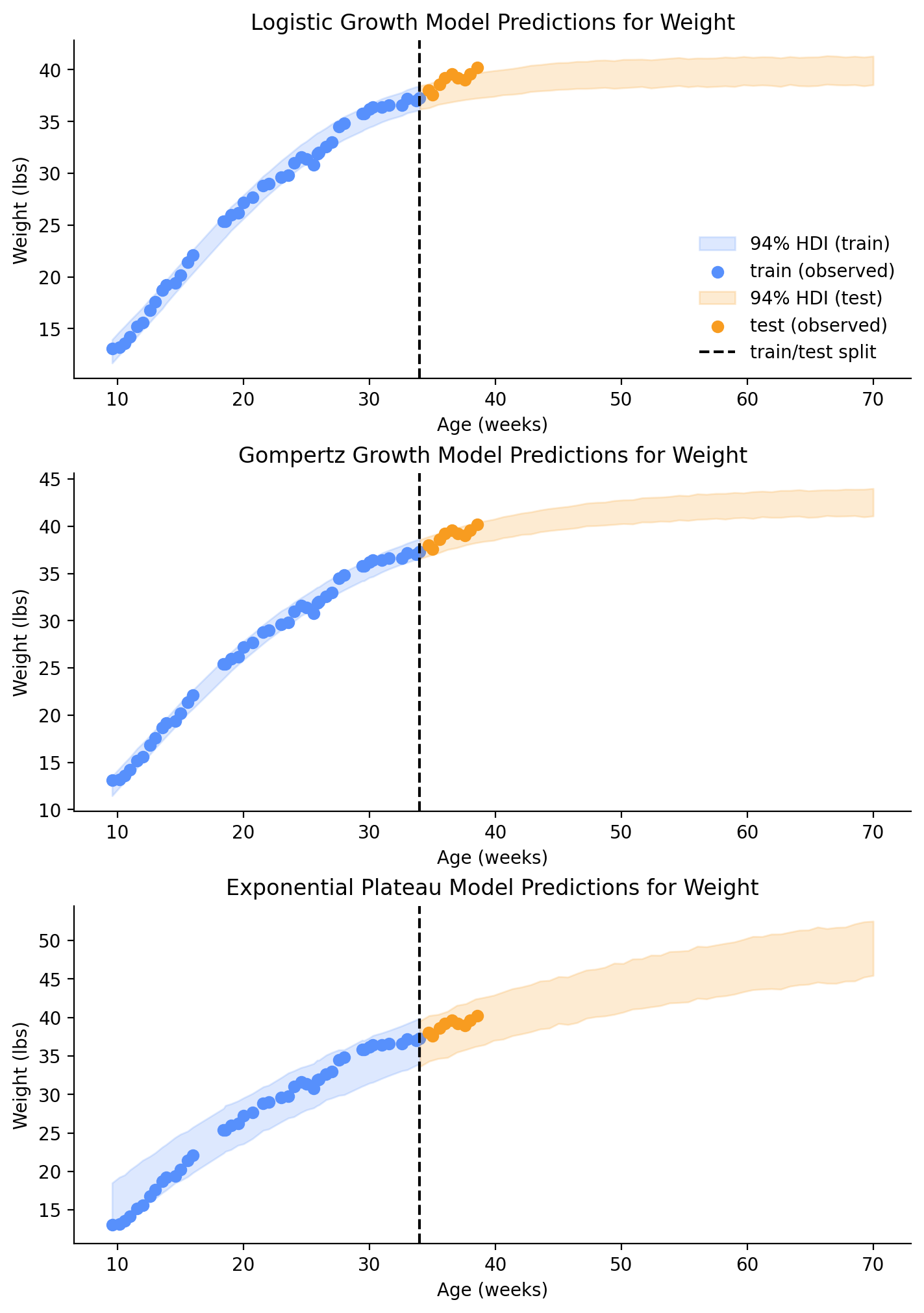
return axLooking at the plots in Figure 7, we can see that the testing data is already starting to deviate from the projection in the Logistic Growth model, but the Gompertz Growth model still looks good.
fig, axes = plt.subplots(3, 1, figsize=(7, 10), layout="constrained")
make_plot(
    df_train,
    df_test,
    posterior_predictive_log_train,
    posterior_predictive_log_test_range,
    weeks_test_range,
    "Logistic Growth",
    axes[0],
)
make_plot(
    df_train,
    df_test,
    posterior_predictive_gompertz_train,
    posterior_predictive_gompertz_test_range,
    weeks_test_range,
    "Gompertz Growth",
    axes[1],
    legend=False,
)
make_plot(
    df_train,
    df_test,
    posterior_predictive_exp_train,
    posterior_predictive_exp_test_range,
    weeks_test_range,
    "Exponential Plateau",
    axes[2],
    legend=False,
);
Compare Dog Weight Predictions
Lastly, we can calculate Root Mean Square Error (RMSE) from our test set and samples from the posterior predictive. The testing dataset has some strange trends in it (due to changes in my dog’s appetite and activity, I’m guessing), but we can still use RMSE as a metric of fit. We will update our input data with the ages in our test set and generate new samples.
Code
posterior_predictive_gompertz_test = evaluate_posterior_predictive(
    model=model_gompertz,
    idata=idata_gompertz,
    test_input=df_test["Age (weeks)"],
    random_seed=rng,
)
posterior_predictive_log_test = evaluate_posterior_predictive(
    model=model_log,
    idata=idata_log,
    test_input=df_test["Age (weeks)"],
    random_seed=rng,
)
posterior_predictive_exp_test = evaluate_posterior_predictive(
    model=model_exp,
    idata=idata_exp,
    test_input=df_test["Age (weeks)"],
    random_seed=rng,
)
These samples have values for each chain (4) and draw (1,000):
posterior_predictive_exp_test.posterior_predictive["obs"].sizesFrozen({'chain': 4, 'draw': 1000, 'obs_id': 9})So, we will take the average across chains and draws to give a single predicted value, which we can compare to our original observed data when calculating the MSE.
def calc_rmse(posterior_predictive: az.InferenceData, observed: pd.Series) -> float:
    predicted = posterior_predictive.posterior_predictive["obs"].mean(("chain", "draw")).to_numpy()
    residuals = predicted - observed.to_numpy()
    return np.sqrt(np.mean(residuals**2))
gomp_rmse = calc_rmse(posterior_predictive_gompertz_test, df_test["Weight (lbs)"])
print(f"Gompertz Growth Model RMSE: {gomp_rmse:.2f}")
exp_rmse = calc_rmse(posterior_predictive_exp_test, df_test["Weight (lbs)"])
print(f"Exponential Plateau Model RMSE: {exp_rmse:.2f}")
log_rmse = calc_rmse(posterior_predictive_log_test, df_test["Weight (lbs)"])
print(f"Logistic Growth Model RMSE: {log_rmse:.2f}")Gompertz Growth Model RMSE: 0.59
Exponential Plateau Model RMSE: 0.85
Logistic Growth Model RMSE: 1.12On average, we would expect to see an error of 0.58 lbs when predicting weight in the future with the Gompertz Growth model, 0.86 lbs with the Exponential Plateau model, and 1.12 lbs (!) with the Logistic Growth model. I think these values could be greater if our test data was from the exponential growth period.
Although the Exponential Plateau model seemed to fit the training data more poorly, and has greater uncertainty, it still seems valid for our small testing dataset.
Bayesian inference status:
- Outline Bayesian model
- Select priors that we will use in our Bayesian models for the growth curves
- Check the priors can give us sensical models (without data)
- Run Bayesian inference models
- Evaluate the quality of posteriors
- Evaluate the quality of our models with some reserved recent data
- Determine when we can be more certain which model is right, and what age my dog will reach her final weight
Final Growth Curve Selection
From what we’ve seen thus far, I think the Gompertz Growth model fits our data best. If we look into the future (Figure 8), at around 60 weeks, the separation between the Gompertz Growth and Logistic Growth models will have stabilized. If one of those models is correct, my dog’s weight will have stabilized too! I’ll make a follow-up post a bit later (April 2024) to see if my dog’s weight is between 41.6 - 43.9 lbs.
Code
posterior_predictive_gompertz_all = evaluate_posterior_predictive(
    model=model_gompertz,
    idata=idata_gompertz,
    test_input=weeks_range,
    random_seed=rng,
)
posterior_predictive_log_all = evaluate_posterior_predictive(
    model=model_log,
    idata=idata_log,
    test_input=weeks_range,
    random_seed=rng,
)
posterior_predictive_exp_all = evaluate_posterior_predictive(
    model=model_exp,
    idata=idata_exp,
    test_input=weeks_range,
    random_seed=rng,
)
Code
fig, ax = plt.subplots(figsize=(7, 5), layout="constrained")
az.plot_hdi(
    x=weeks_range,
    y=posterior_predictive_exp_all.posterior_predictive["obs"],
    hdi_prob=0.94,
    color="C0",
    fill_kwargs={"alpha": 0.3, "label": "94% HDI (Exponential Plateau)"},
    smooth=False,
    ax=ax,
)
az.plot_hdi(
    x=weeks_range,
    y=posterior_predictive_log_all.posterior_predictive["obs"],
    hdi_prob=0.94,
    color="C1",
    fill_kwargs={"alpha": 0.3, "label": "94% HDI (Logistic Growth)"},
    smooth=False,
    ax=ax,
)
az.plot_hdi(
    x=weeks_range,
    y=posterior_predictive_gompertz_all.posterior_predictive["obs"],
    hdi_prob=0.94,
    color="C2",
    fill_kwargs={"alpha": 0.3, "label": "94% HDI (Gompertz Growth)"},
    smooth=False,
    ax=ax,
)

ax.scatter(
    df_train["Age (weeks)"],
    df_train["Weight (lbs)"],
    label="Observed (training)",
    color="0.4",
)
ax.scatter(
    df_test["Age (weeks)"],
    df_test["Weight (lbs)"],
    label="Observed (testing)",
    color="0.5",
)

plt.legend(frameon=False)
ax.set_xlabel("Age (weeks)")
ax.set_ylabel("Weight (lbs)")
ax.set_xlim(left=0)
ax.set_ylim(bottom=0);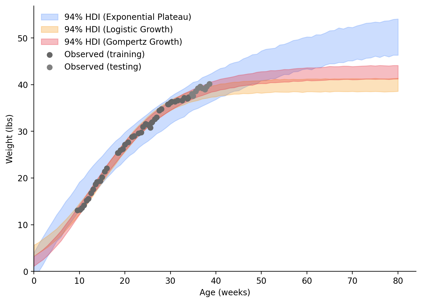
Bayesian inference status:
- Outline Bayesian model
- Select priors that we will use in our Bayesian models for the growth curves
- Check the priors can give us sensical models (without data)
- Run Bayesian inference models
- Evaluate the quality of posteriors
- Evaluate the quality of our models with some reserved recent data
- Determine when we can be more certain which model is right, and what age my dog will reach her final weight
Non-linear Least Squares
Well, that ended up much longer than I thought, but I hope you’re still with me. We will quickly fit the same models using Non-linear Least Squares using scipy’s curve_fit() and plot confidence bands with the help of the uncertainties package.
curve_fit() accepts a function (in the style that we already defined above for each model), independent data, dependent data, and an optional initial guess of parameters. The initial guess isn’t always needed, but can speed up the process, or allow it to happen at all. I will use the means of our priors from above (I’ll give a closer guess for \(k\) because it really needed it).
uncertainties holds onto numbers with uncertainties. It has its own functions that mimic numpy functions, but are built to handle and carry uncertainty. After running curve_fit(), we’ll pass our optimal parameters and covariance matrix through to get uncertain versions of our parameter fits. Since we have np.exp() in our functions, we will also define new versions of our functions that use unp.exp() instead.
import uncertainties as unc
import uncertainties.unumpy as unp
from scipy.optimize import curve_fit
from uncertainties.core import AffineScalarFunc
def logistic_growth(x, ym, y0, k):
# https://www.graphpad.com/guides/prism/latest/curve-fitting/reg_logistic-growth.htm
if isinstance(ym, AffineScalarFunc):
return ym * y0 / ((ym - y0) * unp.exp(-k * x) + y0)
else:
return ym * y0 / ((ym - y0) * np.exp(-k * x) + y0)
def gompertz(x, ym, y0, k):
# https://www.graphpad.com/guides/prism/latest/curve-fitting/reg_gompertz-growth.htm
if isinstance(ym, AffineScalarFunc):
return ym * (y0 / ym) ** (unp.exp(-k * x))
else:
return ym * (y0 / ym) ** (np.exp(-k * x))
def exp_plat(x, ym, y0, k):
# https://www.graphpad.com/guides/prism/latest/curve-fitting/reg_exponential-plateau.htm
if isinstance(ym, AffineScalarFunc):
return ym - (ym - y0) * unp.exp(-k * x)
else:
return ym - (ym - y0) * np.exp(-k * x)def least_squares_fit(
model_func,
model_name,
train_data=df_train,
test_data=df_test,
input_data=weeks_range,
ax=None,
legend=True,
):
if ax is None:
ax = plt.gca()
guess = [45, 1.75, 0.5]
params, params_covariance = curve_fit(
model_func,
train_data["Age (weeks)"],
train_data["Weight (lbs)"],
guess,
)
print(f"{model_name} (Least Squares)")
print(f"ym: {params[0]:.2f}\ny0: {params[1]:.2f}\nk: {params[2]:.2f}\n")
ym, y0, k = unc.correlated_values(params, params_covariance)
px = input_data
py = model_func(px, ym, y0, k)
nom = unp.nominal_values(py)
std = unp.std_devs(py)
# Plot data and best fit curve.
ax.scatter(
data=train_data,
x="Age (weeks)",
y="Weight (lbs)",
s=10,
zorder=10,
color="0.4",
label="Observed (training)",
)
ax.scatter(
data=test_data,
x="Age (weeks)",
y="Weight (lbs)",
s=10,
zorder=10,
color="0.5",
label="Observed (testing)",
)
# plot the nominal value
ax.plot(px, nom, c="C1")
# Add 95% Confidence Interval band
ax.fill_between(
px,
nom - 2 * std,
nom + 2 * std,
alpha=0.6,
color="C1",
label="95% Conf. Int.",
)
if legend:
ax.legend(frameon=False)
ax.set_xlabel("Age (weeks)")
ax.set_ylabel("Weight (lbs)")
ax.set_title(model_name)
# Calculate residuals, RMSE of test set
predicted = model_func(np.asarray(df_test["Age (weeks)"]), *params)
observed = np.asarray(df_test["Weight (lbs)"])
residuals = predicted - observed
mse = np.mean(residuals**2)
rmse = np.sqrt(mse)
print(f"RMSE: {rmse:.2f}\n")Code
fig, axes = plt.subplots(3, 1, figsize=(7, 10), layout="constrained")
least_squares_fit(
    model_func=logistic_growth,
    model_name="Logistic Growth",
    ax=axes[0],
)
least_squares_fit(
    model_func=gompertz,
    model_name="Gompertz Growth",
    ax=axes[1],
    legend=False,
)
least_squares_fit(
    model_func=exp_plat,
    model_name="Exponential Plateau",
    ax=axes[2],
    legend=False,
)
Logistic Growth (Least Squares)
ym: 40.13
y0: 4.63
k: 0.14
RMSE: 1.04
Gompertz Growth (Least Squares)
ym: 42.74
y0: 2.20
k: 0.09
RMSE: 0.58
Exponential Plateau (Least Squares)
ym: 49.51
y0: -9.92
k: 0.05
RMSE: 0.45
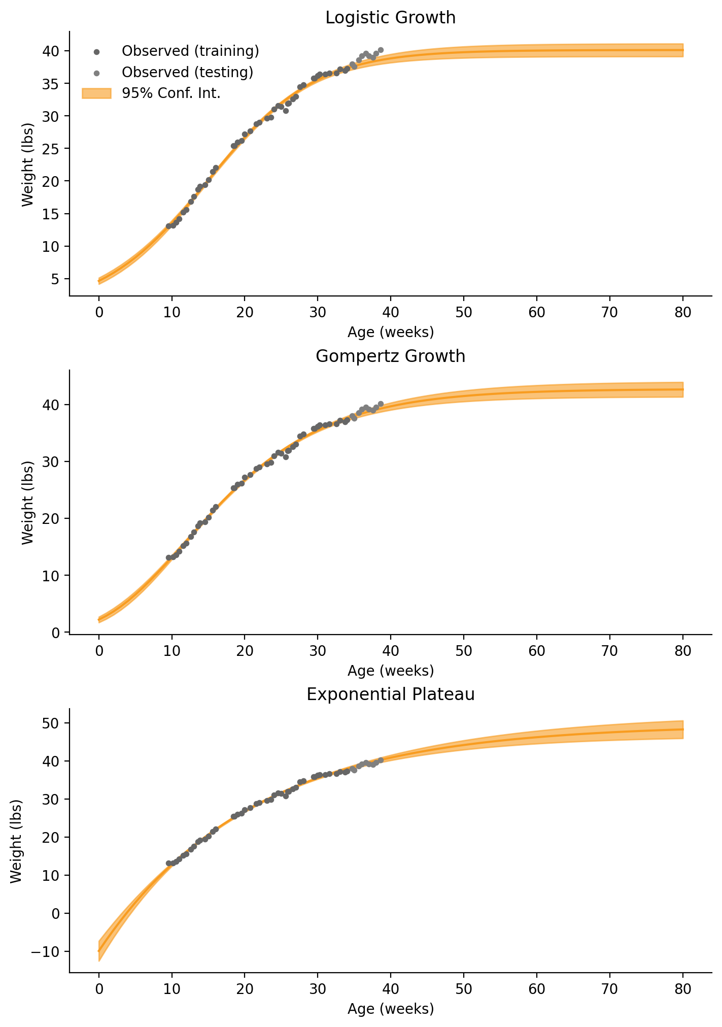
When comparing the Least-Squares estimates and the means of our Bayesian posteriors, the estimates for \(Y_M\) from Logistic Growth and Gompertz Growth are within 0.3 lbs. The estimate for \(Y_M\) from Exponential Plateau is within 4.6 lbs. The Exponential Plateau fit is pretty true to the data this time.
You may have noticed that this is because it was allowed to fit birthweight (\(Y_0\)) to a negative value! When using our Gamma distribution prior in the Bayesian modeling, we prevented negative birthweights. We could also restrain our parameters when using curve_fit(), too. If you don’t need a fully valid model and only care about predicting future weights, loosening our priors could result in a better fit.
Conclusion
We now have some different growth curve models to verify in a few months. I’m going to follow the Gompertz model for now, and predict my dog will reach 41.6 - 43.9 lbs.
Appendix: Environment Parameters
%watermark -n -u -v -iv -wLast updated: Sat Oct 28 2023
Python implementation: CPython
Python version : 3.11.5
IPython version : 8.16.1
preliz : 0.3.6
xarray : 2023.10.1
numpy : 1.25.2
arviz : 0.16.1
pandas : 2.1.1
matplotlib : 3.8.0
seaborn : 0.13.0
pymc : 5.9.1
uncertainties: 3.1.7
Watermark: 2.4.3